Estimating Effect Size in Meta-analysis in the Presence of Publication Bias and Questionable Research Practices
In this report, we aim to reproduce and expand Maassen's research project. In her project, Maassen evaluated the power of several publication bias tests on studies that have been gone under different questionable research practices. Additionally, she altered the intensity of publication bias in order to asses the volatility of their power's.
This paper investigates the impact of publication bias, two questionable research practices (i.e. optional stopping and selective reporting of dependent variables) and their combination on effect size estimates, coverage and power of fixed effect meta-analysis and heterogeneity estimates of random effects meta-analysis. Additionally, the power of three publication bias tests will be estimated, as well as the effect size estimate adjusted for funnel plot asymmetry and the number of trimmed studies from the trim and fill method.
— Maassen
Beyond fixed- and random-effects estimators, the list of publication bias tests includes:
Simulation Design
Maassen has included a range of parameters in her study. The simulation study has been conducted on all combination of parameters from the list below.
- n ∈ {2, 5}
- Pb ∈ {0., 0.05, 0.5, 1}
- K ∈ {8, 24, 72}
- N
- 75% Small ∈ [6, 21]
- 25% Large ∈ [22, 300]
- μ ∈ {0, 0.147, 0.3835, 0.699375}
- ɑ ∈ 0.05
- QRPs
- None
- Selective Reporting
- Selective Reporting
- Optional Stopping
Starting from the top, the simulation study concerns itself with two main Experiment Setup. One with 2, and another with 5 conditions. The sample size, N, of each study is drawn from a piecewise linear distribution where 75% of samples are from [6, 21], and the rest are spreading uniformly between 22 and 300. In addition, true means, μ, of treatment conditions varies between 4 pre-calculated effect size representing studies with small, medium and large power.
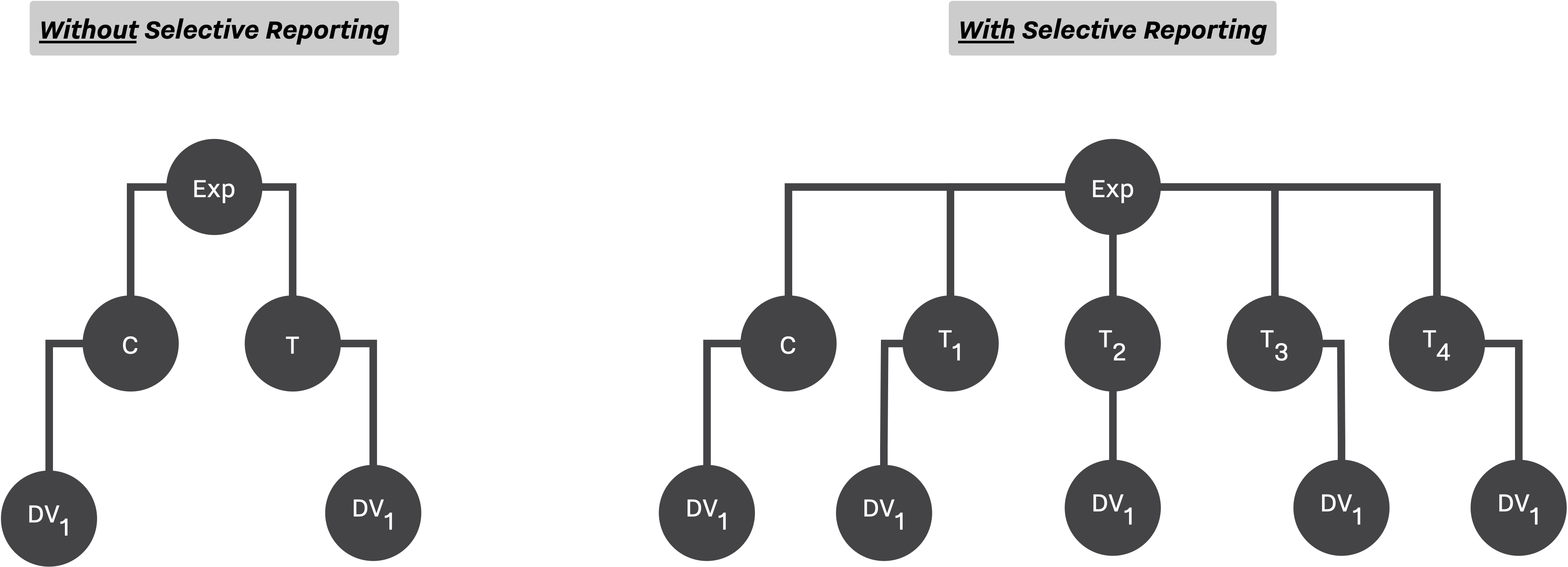
In terms of QRPs, two main methods have been utilized, Selective Reporting, and Optional Stopping. While the optional stopping has been applied on both study designs (at most 3 times, adding ⅓ ⨉ N new observations), the selective reporting can only be applied on the design with 5 conditions (selecting the outcome with minimum p-value).
Finally, after simulating K studies, Maassen applied both meta-analytic methods, and publication bias estimators, and reported their performance.
SAM's Configuration
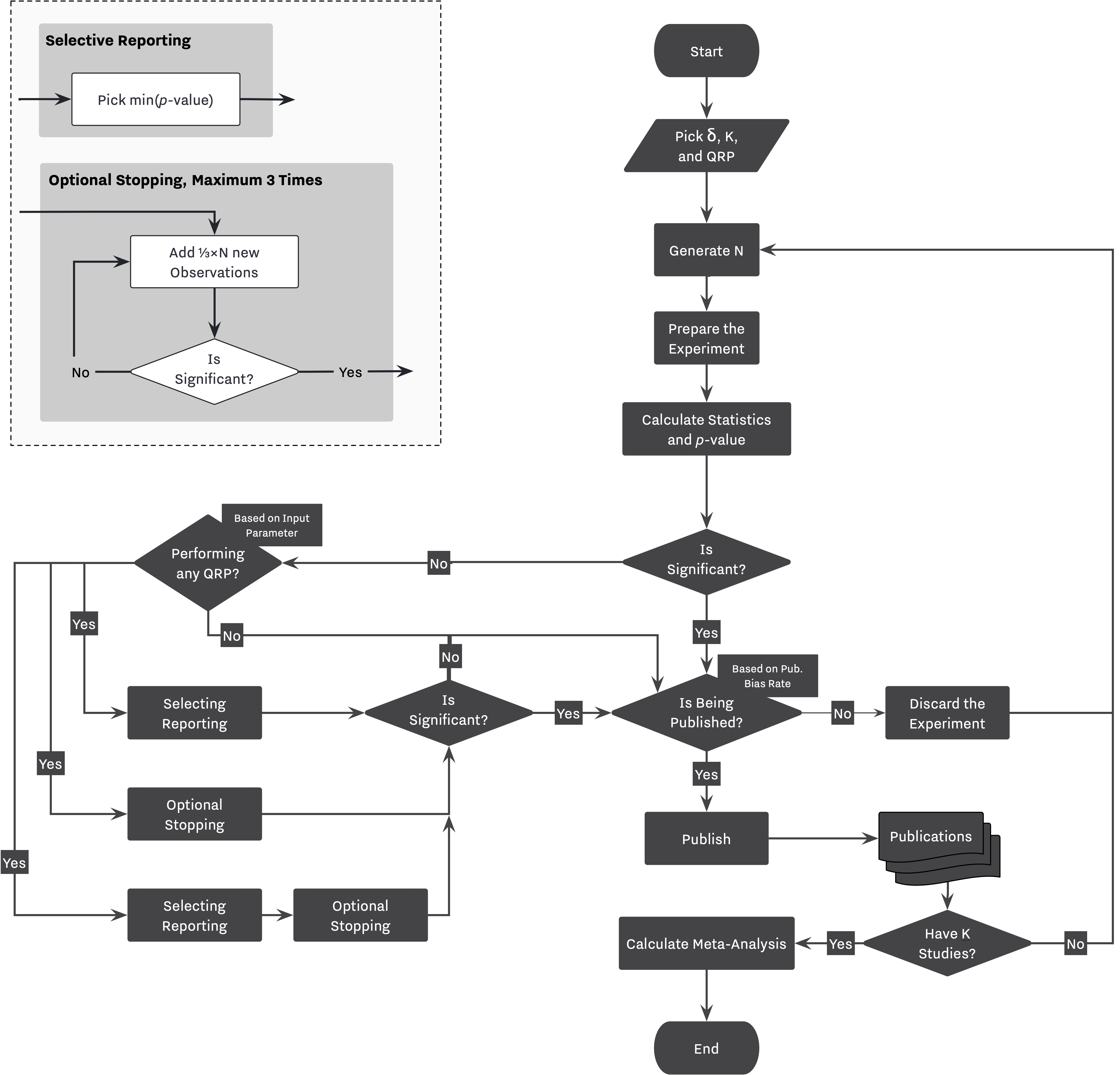
As discussed in other examples, visualizing the simulation flow helps us translate our design to SAM's configuration, Figure 2. While the right-hand side of the flowchart shows the main decision workflow, the left-side mainly describes the process of applying different QRPs based on specific simulation configurations.
Decision Strategy
As we discussed, selective reporting is being applied using the decision strategy module. The Researcher will either select the only available outcome if there is only one primary outcome (ie., no selective reporting), or she will select an outcome with minimum p-value in the presence of selective reporting, line 4.
In cases where the Researcher is equipped with optional stopping, she will decide to apply the method if the selected outcome is not significant, line 5. Finally, if optional stopping has been applied more than once on a study, the last result will be selected, line 6.
Configuration: Decision Strategy
1 2 3 4 5 6 7 8 9 10 11 12 | |
1 2 3 4 5 6 7 8 9 10 11 12 | |
Hacking Strategy
We can configure our hacking strategy as follows. Notice the repetition of decision and selection policies at highlighted lines. This configuration mimics the behavior of "peeking at minimum p-value after each step". After addition of ⅓ ⨉ N, the Researcher selects the outcome with minimum p-value, and if the selected outcome is significant, she stops and reports the outcome, if not, she continues adding another batch of observations, and repeat this process at most 3 times.
Configuration: Hacking Strategy
1 2 3 4 5 6 7 8 9 10 11 12 13 14 15 16 17 18 19 20 21 22 23 24 25 26 27 28 29 30 31 32 33 34 35 36 37 38 39 40 41 42 43 44 45 46 47 48 | |
Data, Test, and Effect Strategy
The combination of Decision Strategy and Hacking Strategy configurations will simulate the process described in Figure 2. Configurations for Data, Test, and Effect strategies have been discussed in more detail in Bakker et al., 2012 example.
Configuration: Data Strategy
1 2 3 4 5 6 7 8 9 10 11 12 13 14 15 16 17 18 19 20 | |
1 2 3 4 5 6 7 8 9 10 11 12 13 14 15 16 17 18 19 20 | |
Configuration: Test Strategy
1 2 3 4 5 6 7 8 9 10 11 12 13 | |
Configuration: Effect Strategy
1 2 3 4 5 6 7 8 9 10 | |
Journal
In the case of Maassen, we need to induce different level of publication bias on our selection procedure. Moreover, we need to calculate a set of meta-analysis and publication bias tests after maxing-out the publications pool. These parameters can be set as follow:
Journal: Publication Bias
1 2 3 4 5 6 7 8 9 10 11 12 13 14 15 16 17 18 19 20 21 22 23 24 25 26 27 28 29 30 31 32 33 34 35 36 37 38 39 40 41 | |
Extended Simulation
In the case of Maassen's simulation, we decided to extend the simulation by covering full range of publication bias, Pb, and true effect size, μ. This extension does not change our main body of configuration. We only need to generate more configuration files with different values of Pb, and μ.
- μ ∈ [0, 1]
- Pb ∈ [0., 1.]
Figures 3–8 illustrate our results in the form of contour plots. The x-axis corresponds to the range of true effect sizes, and y-axis shows the publication bias level, finally contour regions represent the level of bias, or power of our tests.
Staring by the proportion of significant results in our outcomes pool, we notice a regular and expected pattern of higher proportion of significant results with higher true effect sizes and higher rate of publication bias, ie., the yellow region of each plot. Moreover, we see a clear shrinkage in the size of this region as we lower ɑ. Furthermore, notice the growth of the darker regions in lower effect sizes; which can be seen as the influence of lowering ɑ on diminishing the chance of finding significant results with lower true effect sizes.

Looking at the level of effect size bias, we observe higher bias in studies with 5 dependent variables. Moreover, notice the minor negligible effect of our QRPs on the level of bias. This is inline with our results from Bakker et al., 2012 where we concluded that the source of biases is the number of replications, and not the QRPs.

Figure below visualizes the accuracy of random-effect estimate's of the effect size. As we expected, the random-effect estimate improves as we increase K, and declines as we introduce more dependent variables.

As shown below, power of Egger's test consistently improves as we add more publications to our pool, K. Moreover, as expected, we can observe the correlation of higher power with the increase of the publication bias rate. Notice the slight increase of the yellow region as we lowers ɑ, and add more dependent variables. Furthermore, as we discussed in Bakker et al., 2012, we observe a high rate of false positive in simulations with low publication bias rate.

Begg's Rank Correlation Test is an another test for detecting publication bias. As stated by Begg et al.4, the test has a fair power with K > 75, and expected to have lower power with lower K's. While we only simulated pools of publications with K = 72, we can observe the increase in Begg's test power as we increase K. It is worth mentioning that Begg's test performs better than Egger's test in terms of false positives. This can be seen by comparing the size of yellow regions within lower half of each plot, as we see much smaller confidence in reporting publication bias when the true publication bias is lower.

Test Of Excess of Significant Findings [In Progress]
Finally, we measured the power of Test Of Excess of Significant Findings. Figure below shows the results of this measure across our parameters landscape. We are quite surprised with the test, and cannot quite make sense of it yet! Further explanation will follow!

-
Matthias Egger, George Davey Smith, Martin Schneider, and Christoph Minder. Bias in meta-analysis detected by a simple, graphical test. BMJ, 3157109:629–634, 1997. ↩
-
John PA Ioannidis and Thomas A Trikalinos. An exploratory test for an excess of significant findings. Clinical Trials: Journal of the Society for Clinical Trials, 43:245–253, jun 2007. URL: https://doi.org/10.1177%2F1740774507079441, doi:10.1177/1740774507079441. ↩
-
Sue Duval and Richard Tweedie. Trim and fill: a simple funnel-plot–based method of testing and adjusting for publication bias in meta-analysis. Biometrics, 562:455–463, 2000. URL: https://onlinelibrary.wiley.com/doi/abs/10.1111/j.0006-341X.2000.00455.x, arXiv:https://onlinelibrary.wiley.com/doi/pdf/10.1111/j.0006-341X.2000.00455.x, doi:10.1111/j.0006-341X.2000.00455.x. ↩
-
Colin B. Begg and Madhuchhanda Mazumdar. Operating characteristics of a rank correlation test for publication bias. Biometrics, 504:1088–1101, 1994. URL: http://www.jstor.org/stable/2533446. ↩↩