Attention

Please check out Abdol et al., 2021¹ for the updated version of this project. In addition, you can find all the codes, and analysis on GitHub.

The Rules of the Game Called Psychological Science²

In this report, we will attempt to discuss the replication and reproduction of the simulation study conducted by Baker et al., 2012². The simulation is designed to recreate a common routine of applying a set of questionable research practices, and consequently evaluate their effects on the observed effect size bias, and chance of finding significance results.

Experiment Design / Model Description

As described by Bakker, the simulation study is concerned about 4 distinct strategies as follow:

Strategy 1. Perform one large study (with N as the sample size) with sufficient power and publish it.

Strategy 2. Perform one large study and use some of the QRPs most popular in psychology (John et al., 2012). These QRPs may be performed sequentially until a significant result is found: - Test a second dependent variable that is correlated with the primary dependent variable (for which John et al. found a 65% admittance rate) - Add 10 subjects (sequential testing; 57% admittance rate) - Remove outliers (|Z| > 2) and rerun analysis (41% admittance rate)

Strategy 3. Perform, at most, five small studies each with (N/5) as sample size. Players may stop data collection when they find a significant result in the expected direction and only publish the desired result (the other studies are denoted “failed”; 48% admittance rate).

Strategy 4. Perform, at most, five small studies and apply the QRPs described above in each of these small studies if the need arises. Players may report only the first study that “worked.”

— Bakker et al., 2012

Two main distinguishing factors in the simulation are sample size, N, and whether the pre-defined set of QRPs are applied on the study. When it comes to sample sizes, Bakker defines two size classes, small and large. Number of observations in small studies can be a value from {5, 10, 20}, and number of observation in large studies can be either of {25, 50, 100}. Basically, large studies are 5 times larger than small studies. Another difference between small, and large studies is the repetitive nature of conducting small studies. In strategy 3 and 4, each trial is almost an exact replication of the main study — that might or might not have been gone through the QRP procedure. Results from these trials will be collected and at the end, the researcher will get a chance to report the most desirable outcome.

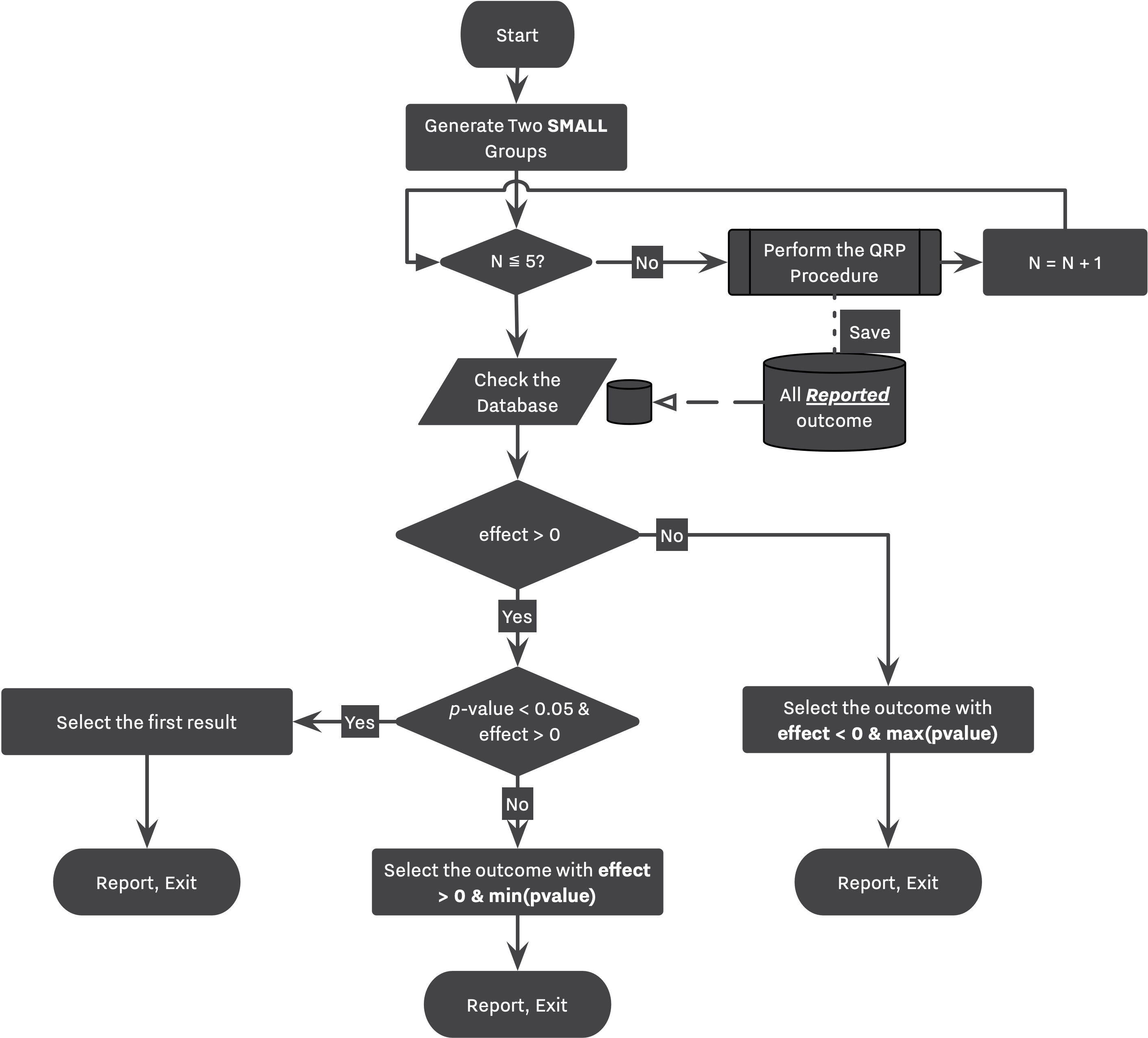
Following flowcharts are visualizing the simulation workflow designed by Bakker. Figure 1 is an equivalent of 1st and 2nd strategies while Figure 2 showcases 3rd and 4th strategies. Notice the "Perform the QRP Procedure" step in Figure 2 where a study goes through the entire process described in Figure 1 labeled as "QRP Procedure".

Figure 1. Flowchart describing Strategy 1, and 2. In the case of Strategy 1, the simulation does not enter the QRP Procedure and reports the first dependent variable.

Figure 2. Flowchart describing Strategy 3, and 4. In the case of Strategy 3, the simulation skips the QRP Procedure but still collects the final outcome from each replication attempts.

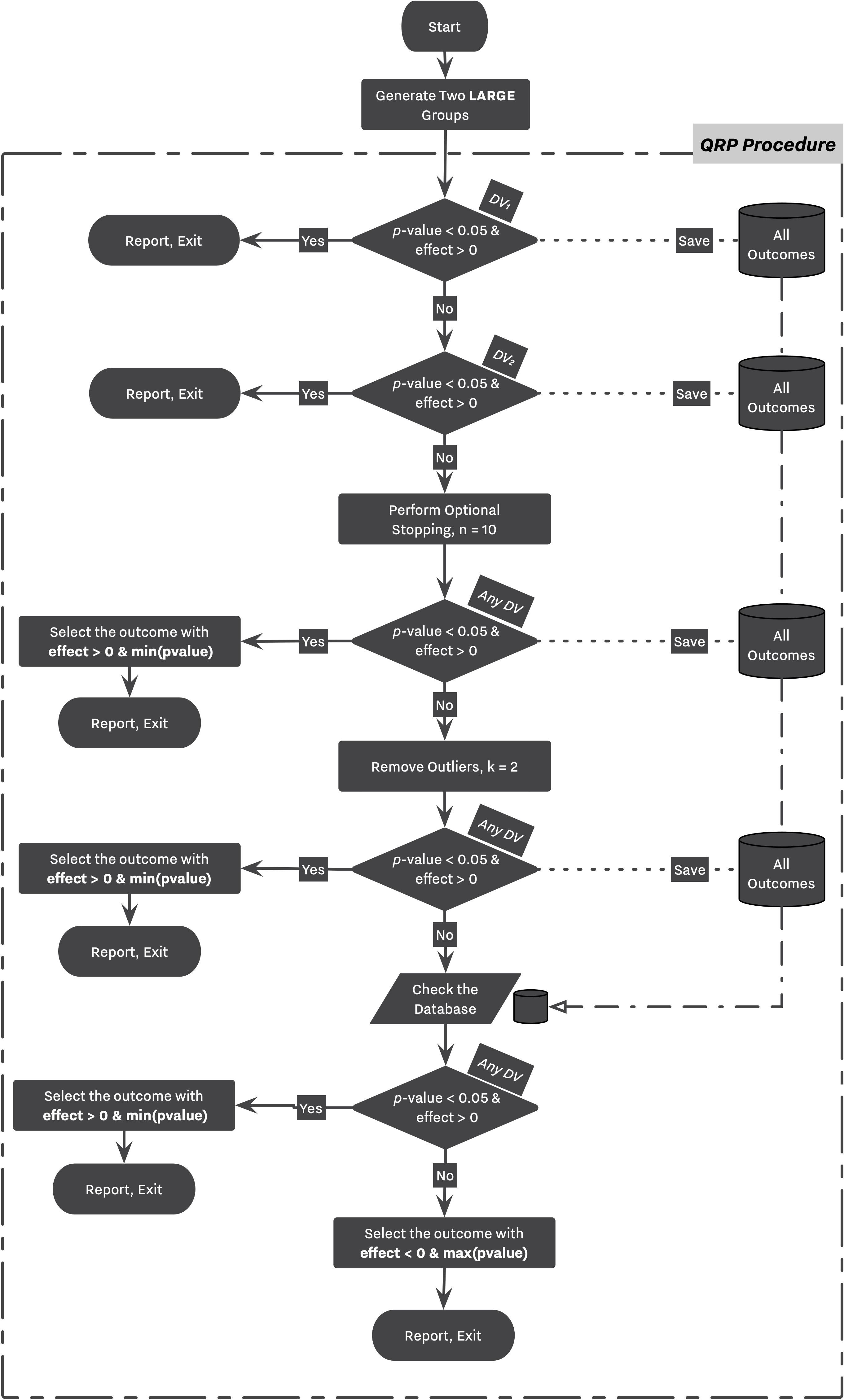
There are several QRPs involved in strategies 2 and 4.

• Every small or large study might go under the Selective Reporting process in which the researcher evaluates and reports the secondary outcome, if she does not find the primary outcome satisfactory.

• Every small or large study might go under the Optional Stopping routine in which the researcher adds 10 new subjects to each DV, and re-calculates her statistics in a quest to find a desirable result.

• Every study might go under the Outliers Removal process in which the researcher attempts to remove all subjects farther than 2 standard deviation from the sample mean in a quest to find a desirable result.

• In large studies, a simulation will stop as soon as the researcher find a significant result with positive effect. However, in small studies, while the researcher reports her finding after performing the set of QRPs (”QRP Procedure” in Fig. 1), she continues to repeat the same routine 5 times, and collects the outcome of each replication,

  • Later in the simulation, as shown in Fig 2., she will select the appropriate outcome from the pool of outcomes collected from all replications.

  • → Strategy 3 follows the same logic with the only difference that each replication doesn’t go through the QRP routines, however, the researcher will still review her finding after performing 5 exact replications.

Besides individual strategies, Bakker et al., explored a wide range of parameters in order to capture the influence of their design. The list of parameters can be found below:

• μ ∈ [0, 1]
• N ∈ {5, 10, 20, 25, 50, 100}
  • Small class, {5, 10, 20}
  • Large class, {25, 50, 100}
• m, n = 2
• 4 scenarios/strategies
• 2 with QRP
• 2 without QRP

The rest of this article focuses on simulating Bakker’s study using SAM, and consequently comparing two approach with each other. Further in the report, we will build on top of Bakker's study in order to investigate the nature of observed biases in more detail.

SAM Configuration

In order to recreate Bakker's simulation using SAM, we start by planning Researcher's Workflow and translating that into a configuration file.

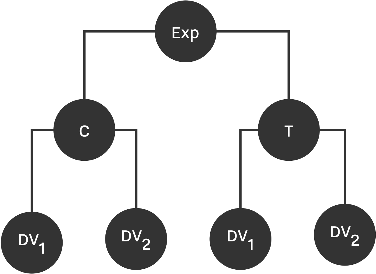
Bakker's experiment is a 2x2 factorial design consists of two groups, Control (C) and Treatment (T) each measuring two dependent variables, as shown in Figure below. The sample population is a multivariate normal distribution with mean of $\hat{0}$ for control group, and $\hat{\mu}$ for treatment group; and standard deviation of $1$, and $0.5$ covarinace between dependent variables. Therefore, $DV_{i} \in MN(\hat{\mu}, \Sigma)$ where $\hat{\mu} = (0, 0, \mu, \mu)$ and

$$\Sigma = \begin{bmatrix} 1 & 0.5 & 0 & 0 \\ 0.5 & 1 & 0 & 0 \\ 0 & 0 & 1 & 0.5 \\ 0 & 0 & 0.5 & 1 \end{bmatrix}$$

This design can be expressed using a Linear Model data strategy as follow:

Configuration: Data Strategy

{
  ...
  "experiment_parameters": {
    "n_obs": 20,
    "n_conditions": 2,
    "n_dep_vars": 2,
    "data_strategy": {
      "name": "LinearModel",
      "measurements": {
          "dist": "mvnorm_distribution",
          "means": [0, 0, μ, μ],
          "sigma": [[1.0,   0.5,   0.0,   0.0],
                    [0.5,   1.0,   0.0,   0.0],
                    [0.0,   0.0,   1.0,   0.5],
                    [0.0,   0.0,   0.5,   1.0]]
    }
  }
  ...
}

Bakker's Researcher uses TTest to asses the significant of its findings. This choice can be expressed with Test Strategy's setting as follow:

Configuration: Test Strategy

{
  ...
  "experiment_parameters": {
    ...
    "test_strategy": {
      "name": "TTest",
      "alpha": 0.05,
      "alternative": "TwoSided",
      "var_equal": true
    }
  }
  ...
}

For effect size measure, Bakker computed the standardized effect size different between two effect. In order to equip SAM with this method, we can use the following configuration of the Effect Strategy:

Configuration: Effect Strategy

{
  ...
  "experiment_parameters": {
    ...
    "effect_strategy": {
      "name": "StandardizedMeanDifference"
    }
  }
  ...
}

After fully configuring Experiment's parameters, we can start translating the simulation logic from a Research Workflow to Decision Strategy's configuration, and thereafter preparing the list of Hacking Strategies.

Strategy 1, and 3 (Without QRPs)

Hacking Strategy

In 1st and 3rd strategies, researchers will NOT commit any QRPs, therefore the probability_of_being_a_hacker should be set to 0. This is enough for configuring a researcher who does not explore the Hacking Workflow.

Decision Strategies

Following the workflow depicted in Figure 1, we are able to set different decision and selection policies in place for the researcher to achieve the exact path described by Bakker.

The researcher always starts by checking the primary outcome, if the selected outcome is not significant and does not have a positive effect (i.e."initial_selection_policies": [["id == 2"]]), she executes the first hacking strategy. Since in 1st and 3rd strategies, we are not performing any QRPs, this path will not be taken.

In the case of small studies, the researcher will replicate 5 exact studies. At the end of each replication, the researcher stores the first outcome variable (as indicated by initial_selection_policies) in a dataset of All Reported Outcome, Figure 2. Finally, she revisits this dataset, and chooses the most desirable outcome among them. Her preferences can be seen under between_replications_selection_policies parameter. This setup is in place to capture the main idea behind Bakker's simulation, that is, "beneficial to a researcher to run 5 small studies instead of one large study."

Configuration: Decision Strategy

{
  ...
  "researcher_parameters": {
    ...
    "probability_of_being_a_hacker": 0,
    "decision_strategy": {
      "name": "DefaultDecisionMaker",
      "initial_selection_policies": [
        ["id == 2"]
      ],
      "will_start_hacking_decision_policies": ["effect < 0", "!sig"],
      "between_hacks_selection_policies": [
        ["effect > 0", "min(pvalue)"],
        ["effect < 0", "max(pvalue)"]
      ],
      "stashing_policy": ["all"],
      "between_replications_selection_policies": [
        ["effect > 0", "sig", "first"],
        ["effect > 0", "min(pvalue)"],
        ["effect < 0", "max(pvalue)"]
      ],
      "will_continue_replicating_decision_policy": [""],
      "submission_decision_policies": [""],
    }
  ...
  }
}

Strategy 2, and 4 (With QRPs)

Hacking Strategies

In 2nd and 4th strategies, the researcher will execute at least one of the listed strategies. After each QRP, the researcher gets to select an outcome from the altered Experiment, after her selection, she can decide on whether she is going to stop there, or applies the next hacking strategy. In Bakker’s case, the selection → decision is simple. The researcher selects the outcome with positive effect and minimum p-value; then, she checks the availability desirability of the selected outcome, if the outcome is not desirable, she executes the next QRP. These settings are highlighted in the following configuration.

Configuration: Hacking Strategy

{
  "researcher_parameters": {
    "hacking_strategies": [
      [
        {
          "name": "OptionalStopping",
          "target": "Both",
          "max_attempts": 1,
          "n_attempts": 1,
          "num": 10
        },
        [
          ["effect > 0", "min(pvalue)" ]
        ],
        ["effect < 0", "!sig"]
      ],
      [
        {
          "name": "OutliersRemoval",
          "target": "Both",
          "max_attempts": 1,
          "min_observations": 1,
          "multipliers": [2],
          "n_attempts": 1,
          "num": 100,
          "order": "random"
        },
        [
          ["effect > 0", "min(pvalue)" ]
        ],
        ["effect < 0", "!sig"]
      ]
    ]
  }
}

Decision Strategy

In Bakker’s simulation, the decision making process between strategies with and without QRPs are very similar. The main research workflow stays intact as shown in Figure 1, and 2. However, now that researchers can commit any QRPs, they will need to choose between all altered outcomes. Bakker’s players tend to collect their findings — regardless of being QRPed — throughout the simulation, and select the most desirable one at the end of their research. This process is shown in Figure 1 with dashed lines transferring results to a temporary dataset, and finally selecting for the most desirable outcome from the temporary database.

As discussed, this process can be simulated in SAM as well. The stashing_policy parameter indicates which of the outcomes will be collected by the researcher during its expedition. At the end of the Hacking Workflow, the between_hacks_selection_policies parameter indicates how is the researcher going to select between those outcomes, ie., Hacked DB, or All Outcomes Database as stated in Figure 1.

Configuration File: Decision Strategy

{
  ...
  "researcher_parameters": {
    ...
    "probability_of_being_a_hacker": 1,
    "decision_strategy": {
      "name": "DefaultDecisionMaker",
      "between_hacks_selection_policies": [
        ["effect > 0","min(pvalue)"],
        ["effect < 0","max(pvalue)"]
      ],
      "between_replications_selection_policies": [
        ["effect > 0", "sig", "first"],
        ["effect > 0", "min(pvalue)"],
        ["effect < 0", "max(pvalue)"]],
      "initial_selection_policies": [
        ["id == 2", "sig", "effect > 0"],
        ["id == 3", "sig", "effect > 0"]
      ],
      "stashing_policy": ["all"],
      "submission_decision_policies": [""],
      "will_continue_replicating_decision_policy": [""],
      "will_start_hacking_decision_policies": ["effect < 0", "!sig"]
    }
  ...
  }
}

Results

We start by comparing the results between the original simulation and the reproduced study.

Original vs. Reproduction

Figure 4 compares the results of the original study and the reproduced simulation. As it can be seen, the reproduction simulation — distinguished by points — are mainly agreeing with the original simulation with exception of some minor discrepancies in small studies. In all cases, the reproduction simulation captures more bias in small studies with QRPs.

Figure 4. Comparison between original and reproduced results (using SAM).

The Source of Discrepency

Further investigation led to the finding of a minor bug in Bakker et al., code where a typo resulted in insertion of a wrong large study in the replication pool of small simulation. This polluted the pool of small studies and reduced the overall observed bias, due to the wrongly inserted large study having lower bias among all other small studies. Figure 5, shows the comparison of results from the patched script, and SAM's results. As it is shown, patching Bakker's code accounted for the minor discrepancy and consequently we gets a perfect replication.

Figure 5. Comparison between results from the patched script and results from SAM.

First Extension: α‘s Role

Building on top of Bakker’s simulation and using SAM’s flexibility we can extend their simulation to study the observed effect size bias, ES Bias, under different values of α ∈ {0.0005, 0.005, 0.05}.

The main body of the simulation is identical to the original simulation performed by Bakker. Therefore, we start from the final configuration file and in order to enforce different alpha levels, the only parameters that needs to be changes is test_alpha.

Configuration: Test Strategy

{
  ...
  "experiment_parameters": {
    ...
    "test_strategy": {
      "name": "TTest",
      "alpha": 0.05,
      "alternative": "TwoSided",
      "var_equal": true
    }
  }
  ...
}

By running the simulation under selected range of parameters, we will be able summarize our results for different levels of alpha in Figure 6 and 7. Here we can follow the effect of alpha on probability of finding significance and the amount of induced biased under Bakker’s rules.

Figure 6 shows the chance of finding at least one significant result. As expected, from left to right, the chance of finding significant result — in all cases — increases as we increase α but not so drastically.

Figure 7 shows the level of bias in the estimated effect. The effect of lowering the α on ES bias is not as obvious as it is on the chance of finding significant results. In almost all cases, the largest α leads to less bias in the effect as the true effect size increases. In 4th strategy, where the researcher applies a set of QRPs on small studies, the bias rises even more drastically as we lower α. It’s worth mentioning that the researcher has not adoptted his strategies to the adjusted values of α. In all cases, she still adds 10 new subjects and removes subjects with values further than 2 standard deviations.

Figure 6. Chance of finding a significant result with regards to different values of α.

Figure 7. ES Bias with regards to different values of α.

The effect of α on the chance of finding a significant result and ES bias can be visualized using a heatmap as well. Figure 7 and 8 showcase the trends and patterns more vividly. With regards to chance of finding a significant result, as discussed before, we can see a clear decline as we decrease α. This can be seen by the movement of the dark region (lower probability) to the right side (higher effects).

While we can see a clear change in the probability of finding a significant result, the heatmap of ES bias looks very scattered and with no clear patterns or trends. This is the indication of a non-linear relation between α and ES bias. While decreasing alpha makes it harder to find a significant results, a weak experiment design carries its bias with it anyway.

Effect of Replications

Before we end the first extension, we studied the effect of number of replications in Bakker et al. simulation. Figures below showcase the effect that different number of replications has on the chance of finding significant and also on the bias accumulated in effect size. While these figures might look crowded, the only thing we are trying to emphasize is the fact that more replications lead to more bias in our studies. This can be seen by tracing points' shapes in each plots.

In fact we believe this is the only source of bias in Bakker et al. simulation, and the effect of QRP is minimal in comparison to drastic level of bias induced by only running the same study several times. The next extension put this hypothesis to test by replacing Bakker et al. QRPs with more aggressive methods and parameters.

Chance of Finding Sig.

Chance of finding a significant result with regards to different number of replications.

ES Bias

ES Bias with regards to different number of replications.

Second Extension: More Aggressive QRPs

Another extension of this model could investigate the effect of more aggressive QRPs when stricter α’s are introduced. For instance, we could adjust Optional Stopping such that the researcher adds new subjects one by one until she finds a significance result. Furthermore, the Outliers Removal procedure can be replaced by a Subjective Outliers Removal method where the researcher continuously lowers k and remove corresponding outliers until she finds a significant results. These two changes can be added to the configuration file as following:

Hacking Strategy: Advance Hacker

{
  ...
  "hacking_strategies": [
    [
      {
        "name": "OptionalStopping",
        "target": "Both",
        "prevalence": 0.1,
        "defensibility": 0.1,
        "max_attempts": 1,
        "n_attempts": 10,
        "num": 1,
        "stopping_condition": ["sig"]
      },
      [
        ["effect > 0", "min(pvalue)" ]
      ],
      ["effect < 0", "!sig"]
    ],
    [
      {
        "name": "SubjectiveOutlierRemoval",
        "min_observations": 5,
        "range": [2, 4],
        "step_size": 0.5,
        "target": "Both",
        "prevalence": 0.1,
        "defensibility": 0.1,
        "stopping_condition": ["sig"]
      },
      [
        ["effect > 0", "min(pvalue)" ]
      ],
      ["effect < 0", "!sig"]
    ]
  ]
...
}

Figures below show the results of these modifications. As it is shown, while these adjustments introduce slightly more bias into publications; their effect is not as drastic as one would assume. Combining there results with results of previous extension, we are more certain that the effect of QRPs is minimal.

This in fact strengthen Bakker et al. hypothesis by showcasing the immense effect and advantage of running small studies over larger studies. Studies with low sample size are volatile enough that a researcher could easily achieve significant results with unrealistic effect sizes throughout the realistic effect size spectrum.

Chance of finding a significant result with regards to different values of α.

ES Bias with regards to different values of α.

Third Extension: Influence of Publication Bias

In our last extension, we will explore the effect of publication bias on the level of effect size bias; moreover, we investigated the power of Egger's³ test under different publication bias levels.

In order to incorporate the effect of publication bias to our simulation, we equip the Journal module with a Selection Strategies that mimics this effect. The Significant Selection allows us to set adjust the publication bias of the Journal, pub_bias and induce different level of publication bias into our simulation. For this study, we use different values of publication bias, {0., 0.1, ..., 0.9, 1.0}.

Journal: Publication Bias

{
  ...
  "journal_parameters": {
    "max_pubs": k,
    "selection_strategy": {
        "name": "SignificantSelection",
        "pub_bias": p,
        "alpha": ɑ,
        "side": 0,
    },
    "meta_analysis_metrics": [
        {
            "name": "RandomEffectEstimator",
            "estimator": "DL"
        },
        {
            "name": "EggersTestEstimator",
            "alpha": 0.1
        }
    ]
  }
  ...
}

In this setup, we would like to run our meta analysis methods publication pool size of K = 24. This can be done by setting max_pubs parameters of journal_parameters. With this configuration, after journal max-ed out its publications list, it calculates RandomEffectEstimator and EggersTestEstimator, and writes the results into different files for further analysis.

Starting by our general plots, we can observer the effect of publication bias on proportion of significant results in our publications pool.

0.0

0.1

0.2

0.3

0.4

0.5

0.6

0.7

0.8

0.9

1.0

Moreover, the level of bias can be seen below. As expected, raising the publicatoin bias raises the level of bias accross all our configurations, with sharper swell in lower true effect sizes.

0.0

0.1

0.2

0.3

0.4

0.5

0.6

0.7

0.8

0.9

1.0

Figures below showcase the power of Egger's test in detecting publication bias. The average performance of the test is accepetable within most parameter configurations. However, we see large regions of false positives where Egger's test overestimate the presence of the publication bias, especially within smaller true effect sizes. It is also worth mentioning that Egger's test performs quite poorly within a pool of studies with larger sample sizes, L; N = 40, even with publication bias as high as %90.

0.0

0.1

0.2

0.3

0.4

0.5

0.6

0.7

0.8

0.9

1.0

Conclusion

In this example, we discussed the process of translating an existing project into SAM. We started by replicating the original simulation, fine-tunning our configuration and comparing our results. Consequently, after successfully replicating the original results, we built on top Bakker et al., simulation.

In our first extension, we showed that while lowering the alpha decreases the chance of finding significant results it does not necessarily help with the reduction of bias. Moreover, we showed that the number of replications directly influence the level of bias.

In the second extension, we showed that more aggressive QRPs do not proportionally contribute to higher effect size biases. Together with our results from first extension, we believe that the main source of bias in Bakker et al., is the number of replications and the role of QRPs are almost negligible.

In our third and last extension, we investigated the effect of publication bias on the overall bias and the power of Egger’s test in defecting publication bias. We showed that while Egger's test generally provide a good measure of publication bias in the presence of publication bias, it consistently overestimate the level of bias when there is not publication bias is present.

---

1. Amir M. Abdol and Jelte M. Wicherts. Science Abstract Model Simulation Framework. PsyArXiv, 09 2021. URL: https://psyarxiv.com/zy29t, doi:10.31234/osf.io/zy29t. ↩

2. Marjan Bakker, Annette van Dijk, and Jelte M. Wicherts. The rules of the game called psychological science. Perspectives on Psychological Science, 7$6$:543–554, nov 2012. URL: https://doi.org/10.1177%2F1745691612459060, doi:10.1177/1745691612459060. ↩↩

3. Matthias Egger, George Davey Smith, Martin Schneider, and Christoph Minder. Bias in meta-analysis detected by a simple, graphical test. BMJ, 315$7109$:629–634, 1997. ↩

---

Last update: 2021-09-18