Outlier Removal, Sum Scores, and The Inflation of the Type I Error Rate In Independent Samples T Tests: The Power of Alternatives and Recommendations1
This report discusses the process of partially reproducing the simulation study conducted by Bakker et al, 20141. The simulation aims to study effects of removing outliers on Type I error. Besides a regular Linear Model, Bakker et al have simulated data from the General Graded Response Model2. The original study also explores the power of alternative tests, e.g., Yuen's Test3, and Wilcoxon's Test4.
Experiment Design / Model Description
The original study is testing the effects of removing outliers in two main scenarios:
- Non-Subjective Outliers Removal, in which the effect of removing outliers with |Z| > k — **for a fixed *k** — is being measured.
- Subjective Outliers Removal, in which the effect of removing outliers with a variable k ∈ {3, 2.5, 2} is being measured.
Figure 1 shows the flow of two main simulation scenarios. As discussed, by Bakker et al, 2014, the subjective Type I error is calculated based on results of the non-subjective simulation:
Furthermore, we investigated the subjective use of k. This means that a comparison is counted as statistically significant if the test showed a statistically significant difference when all values were included in the sample or when the test showed a statistically significant difference when k is 3, 2.5, or 2. This is comparable with adapting k until a statistically significant p-value is found. This reflects a manner in which researchers can chase for significance (Ioannidis, 2005, 2012), ...
— Bakker et al., 2012, page 5.
As stated by Bakker, this should be equivalent to calculating the subjective Type I Error from the posterior of the non-subjective simulation. We put this theory to test by running a separate simulation for the subjective outliers removal. In fact, in the reproduction simulation we are going to simulate the behavior of a researcher who dynamically reduces k until she finds a significant result.

SAM Configuration
Experiment Parameters and Study Design
In the original study, the data is generated based on two models, Linear Model and General GRM with following parameters:
- different number of items, i ∈ {2, 5, 10, 20, 40}
- different number of options per items, j ∈ {1, 5}
- different difficulty levels, β ∈ {0, 3}
- different sample sizes, N ∈ {20, 40, 100, 500}
- and one ability level, α ∈ 0
Finally, the [Rasch Model]5 is being used as the response function of the GRM:
where \theta_j is j'th examinee ability trait, and \beta_i is the difficulty of item i.
In both scenarios, the study design consists of two groups, and a single dependent variant is being measured in each group, as described in Figure 2.
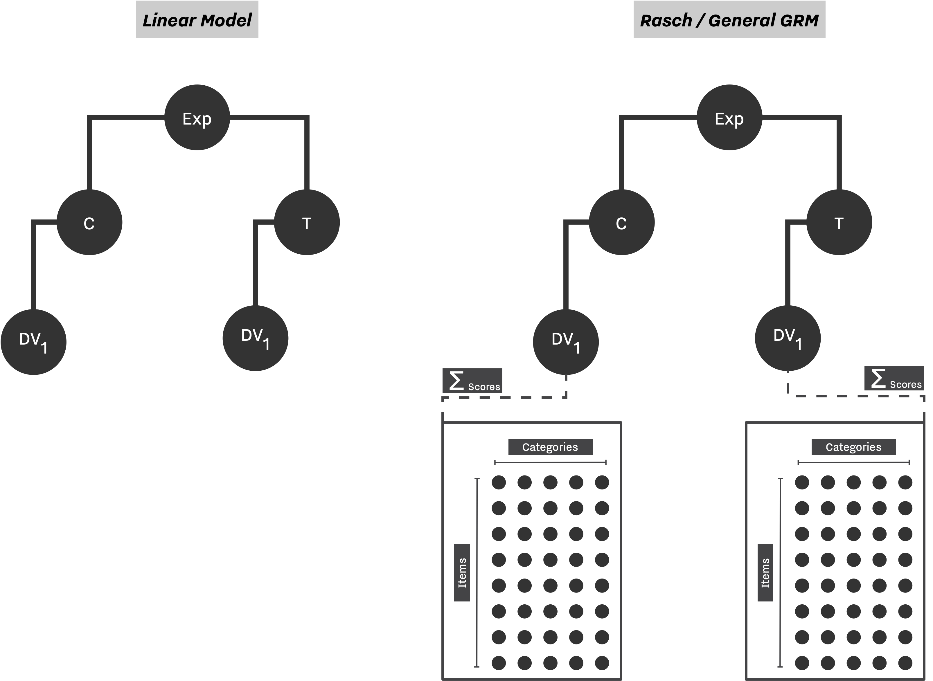
Configurations below showcase how one can express the presented design in SAM. In the case of Linear Model, the setup is simple, we set the data strategy to Linear Model and define a multivariate normal distribution to populate all DVs. For simulating Rasch and GRM model, we use the General Graded Response Model framework, and set appropriate difficulty and ability parameters as shown below:
Configuration: Data Strategy
"experiment_parameters": {
    "n_reps": 1,
    "n_conditions": 2,
    "n_dep_vars": 1,
    "n_obs": 100,
    "data_strategy": {
        "name": "LinearModel",
        "measurements": {
            "dist": "mvnorm_distribution",
            "means": [0, μ],
            "stddevs": 1.0,
            "covs": 0.0
        }
    },
    "test_strategy": {
        "name": "TTest",
        "alpha": 0.05,
        "alternative": "TwoSided",
        "use_continuity": true
    },
    "effect_strategy": {
        "name": "MeanDifference"
    }
}
"experiment_parameters": {
    "n_reps": 1,
    "n_conditions": 2,
    "n_dep_vars": 1,
    "n_obs": 100,
    "data_strategy": {
        "name": "GradedResponseModel",
        "n_items": 40,
        "abilities": {
            "dist": "mvnorm_distribution",
            "means": [
                0,
                μ
            ],
            "stddevs": 1.0,
            "covs": 0.0
        },
        "n_categories": 5,
        "difficulties": {
            "dist": "mvnorm_distribution",
            "means": [
                θ,
                θ,
                θ,
                θ
            ],
            "stddevs": 1.0,
            "covs": 0.0
        },
        "response_function": "Rasch",
    },
    "test_strategy": {
        "name": "TTest",
        "alpha": 0.05,
        "alternative": "TwoSided",
        "use_continuity": true
    },
    "effect_strategy": {
        "name": "MeanDifference"
    }
}
"experiment_parameters": {
    "n_reps": 1,
    "n_conditions": 2,
    "n_dep_vars": 1,
    "n_obs": 100,
    "data_strategy": {
        "name": "GradedResponseModel",
        "n_items": 40,
        "abilities": {
            "dist": "mvnorm_distribution",
            "means": [
                0,
                0
            ],
            "stddevs": 1.0,
            "covs": 0.0
        },
        "n_categories": 2,
        "difficulties": [
            {
                "dist": "normal_distribution",
                "mean": 0,
                "stddev": 1.0
            }
        ],
        "response_function": "Rasch",
    },
    "test_strategy": {
        "name": "TTest",
        "alpha": 0.05,
        "alternative": "TwoSided",
        "use_continuity": true
    },
    "effect_strategy": {
        "name": "MeanDifference"
    }
}
Hacking Strategies
For simulating the Outliers Removal process, we take a different approach than the one we have used for Bakker et al., 2012 simulation. Here, we simulate the outliers removal step before passing the Experiment to the Researcher. This is equivalent to pre-processing the data and then running the final tests and analyses on it.
For this purpose, we are using the pre_processing_methods parameter in researcher_parameters section. Pre-processing steps are similar to normal hacking strategies with the difference that the Researcher does not get to perform a selection → decision sequence after each step. They are being fully applied one after another, and when the list is exhausted, a copy of the modified Experiment will be passed to the Researcher for further analysis.
Configuration: Pre-processing
    "probability_of_being_a_hacker": 0,
    "probability_of_committing_a_hack": 0,
    "hacking_strategies": [""],
    "is_pre_processing": true,
    "pre_processing_methods": [
        {
            "name": "OutliersRemoval",
            "target": "Both",
            "prevalence": 0.5,
            "defensibility": 0.1,
            "min_observations": 5,
            "multipliers": [
                k
            ],
            "n_attempts": 1,
            "num": N,
            "order": "random"
        }
    ]
    "probability_of_being_a_hacker": 0,
    "probability_of_committing_a_hack": 0,
    "hacking_strategies": [""],
    "is_pre_processing": true,
    "pre_processing_methods": [
        {
            "name": "SubjectiveOutlierRemoval",
            "min_observations": 5,
            "prevalence": 0.5,
            "target": "Both",
            "defensibility": 0.1,
            "range": [
                2,
                3
            ],
            "step_size": 0.5,
            "stopping_condition": [
                "sig"
            ]
        }
    ]
Decision Strategies
Neither of the simulation scenarios involve a complicated design making routine compared to Bakker et al., 2012 multistep decision making process. Here, in both cases, we are only interested in reporting the only available dependent variable, and this can be done by setting initial_selection_policies to ["id == 1"] or ["pre-reg"]. With this configuration, the Researcher initializes an Experiment, perform the pre-processing step, and "blindly" submit the only DV to the Journal without altering the experiment.
This simple decision strategy can be used to skip the entire decision workflow, and study the Experiment in its purity without any dynamic interventions from the Researcher.
Configuration: Decision Strategy
"decision_strategy": {
    "name": "DefaultDecisionMaker",
    "initial_selection_policies": [
        [
            "id == 1"
        ]
    ],
    "between_hacks_selection_policies": [[""]],
    "between_replications_selection_policies": [[""]],
    "stashing_policy": [""],
    "submission_decision_policies": [""],
    "will_continue_replicating_decision_policy": [""],
    "will_start_hacking_decision_policies": [""]
}
Results
Original vs. Reproduction
Figure 3 shows the results of removing outliers from a normally distributed sum scores, aka. linear model. This is the equivalent of results showcased in Figure 1 of Bakker et al. 2014. While we didn't overly the results from the original study due to difficulty of extracting the data in compatible format, it can be seen that our results agrees with results form the original study, and we see a similar trends in Type I Error reduction as we increase k.

Similarly, Figure 4 shows the results of removing outliers from Rasch and GRM. Figure 4 is equivalent of results presented in Figure 2, and 3 of Bakker study. We again see a similar trends with respect to increasing k, number of items and higher difficultly.

First Extension: Effect of Publication Bias
As we did with Bakker et al., 2012 study, we demonstrate how we can extend the currently established simulation with a few modification and explore different aspects of the problem using SAM.
In the first extension, we introduce a biased journal to the simulation by modifying the selection strategy of the Journal module as follow:
Configuration: Biased Journal
    "journal_parameters": {
        "max_pubs": 5000,
        "selection_strategy": {
            "name": "SignificantSelection",
            "alpha": 0.05,
            "pub_bias": Pb,
            "side": 0
        }
    }
By varying this configuration, and keeping the rest of the setup intact, we will be able to study the effect of publication bias on our design. Figure 5 shows the results of this modification. As one would expect, we can see higher Type I error in publications as we increase the publication bias rate, from top to bottom. Also, we can see that Type I error rate decreases as we increase the number of items, and examinees, as expected.


Second Extension: Meta-analysis and Bias Level
While we will discuss the power of Egger's Test and several other meta-analysis metrics, and publication bias correction methods in Maassen et al. simulation study, here for the second extension, we focus on the linear model of Bakker et al., 2014 simulation and study the power/accuracy of Egger's Test on two different meta-analysis pool with different size as well as the accuracy of Random Effect estimator, Figure 6 and Figure 7 respectively.
Configuration: Biased Journal
"journal_parameters": {
    "max_pubs": 5000,
    "selection_strategy": {
        "name": "SignificantSelection",
        "alpha": 0.05,
        "pub_bias": Pb,
        "side": 0
    },
    "meta_analysis_metrics": [
        {
            "name": "RandomEffectEstimator",
            "estimator": "DL"
        },
        {
            "name": "EggersTestEstimator",
            "alpha": 0.1
        }
    ]
}


-
Marjan Bakker and Jelte M. Wicherts. Outlier removal, sum scores, and the inflation of the type i error rate in independent samples t tests: the power of alternatives and recommendations. Psychological Methods, 193:409–427, 2014. URL: https://doi.org/10.1037%2Fmet0000014, doi:10.1037/met0000014. ↩↩
-
Fumiko Samejima. Graded Response Model, pages 85–100. Springer New York, New York, NY, 1997. URL: https://doi.org/10.1007/978-1-4757-2691-6_5, doi:10.1007/978-1-4757-2691-6_5. ↩
-
KAREN K. YUEN. The two-sample trimmed t for unequal population variances. Biometrika, 611:165–170, 04 1974. URL: https://doi.org/10.1093/biomet/61.1.165, doi:10.1093/biomet/61.1.165. ↩
-
Frank Wilcoxon. Individual Comparisons by Ranking Methods, pages 196–202. Springer New York, New York, NY, 1992. URL: https://doi.org/10.1007/978-1-4612-4380-9_16, doi:10.1007/978-1-4612-4380-9_16. ↩
-
Susan E Embretson and Steven Paul Reise. Item response theory for psychologists. Maheah. New Jersey: Lawrence Erlbaum Associates, Publishers, 2000. ↩